18 minutes
Charity Bike Rides and Kalman Filters - Part 1
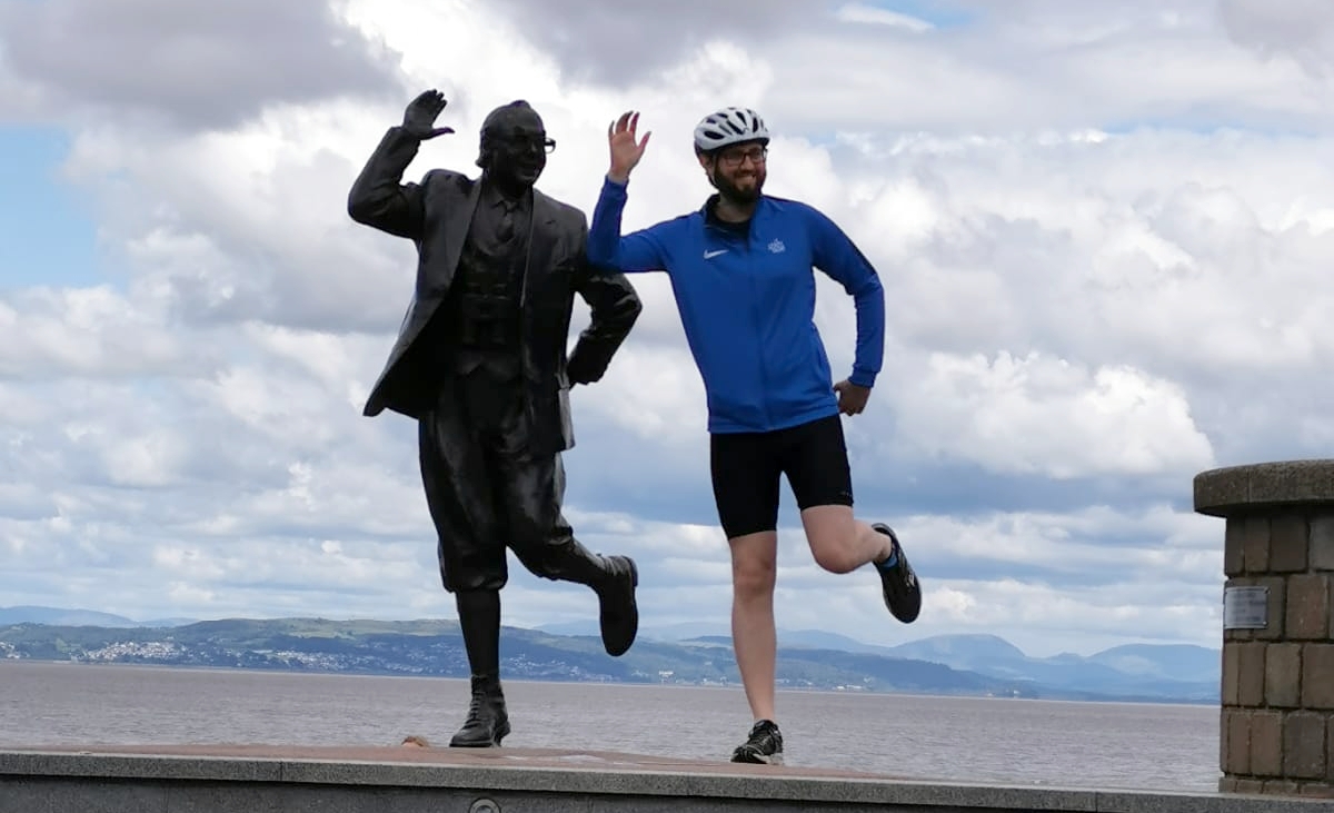
During 2020 at Peak, we used one of our quarterly company events to get away from the screens and raise some money for the charity Fareshare Greater Manchester. Our goal was to travel the length of the UK which we comfortably achieved, whilst raising money for a great cause. I cycled (stopping by a famous local landmark above) recording the journey using a fitness tracker which produces some interesting GPS data that I have not previously had the opportunity to analyse. One of the great things about GPS location data is that it is a perfect way of illustrating the principles of the Kalman filter, a technique widely used in time series analysis. I ended up writing more than I anticipated so I have split this discussion into multiple posts. In this post, I will illustrate the basics of the Kalman filter (having been inspired by previous coverage such as this and this) and how to apply it before in future posts showing extensions with the extended Kalman Filter and an application to real data.
The following series of posts will be a relatively in depth look at the practical application of Kalman filters, with some of the more mathematical steps for my own use as much as anything else, feel free to skip over the linear algebra to look at the code.
Why do we need the Kalman filter?
Fundamentally the Kalman filter helps us to filter a noisy signal such as the one in the left panel below to the much cleaner signal in the right hand panel:
Kalman Filter applied to a noisy signal
The Kalman filter was developed in 1960 by Rudolf Kálmán. One of its first applications was in the Apollo navigation computer used to take humans to the moon (see this article for an overview and the many scientists involved). The Kalman filter is one of several techniques that allows anyone who utters the phrase “it’s not rocket science” to have an eyebrow raised at them. The Kalman filter has a wide variety of applications in guidance, navigation, and control of vehicles and in many time series analysis applications, in fields such as signal processing and econometrics; the latter being where my personal familiarity began.
When we are cycling along we would like to record the path we took to examine it later and so to track where we have cycled we can record it using a GPS receiver in a phone. The fundamental issue is that our “true” position is unknown at any particular point of time and the GPS receiver will be inaccurate, perhaps due to passing through a tunnel, or cycling near a large building. Even under ideal conditions the expected accuracy of GPS is +/-5m on a smartphone, with even worse performance on altitude (which we will ignore for now). To examine how to use the Kalman filter in this situation let’s simplify the problem down to a cyclist who is cycling around a perfectly circular track. This path can be modelled with \(x\) and \(y\) coordinates given by:
We can model this in R and to make our lives easier I have ensured that in 100 time steps the cyclist makes it around the circle:
# Vector of time observations which ensures a perfect circular path
t <- seq(from = 0, to = 2 * pi, length.out = 100)

# Calculate the difference betwee time steps - we will need this later
dt <- t[2] - t[1]

# Equation of a circular path
x <- cos(t)
y <- sin(t)
Now let’s concentrate on how the data from a GPS receiver would look in this example. Every so often the GPS reader records its longitude and latitude. As previously discussed this is a noisy signal so we add a random term to the \(x\) and \(y\) coordinates to produce our GPS readings, with a mean of 0 and standard deviation of 0.05.
# GPS standard deviation
gps_sd <- 0.05

# GPS readings
x_gps <- x + rnorm(length(x), mean = 0, sd = gps_sd)
y_gps <- y + rnorm(length(y), mean = 0, sd = gps_sd)
As in the real world these red points (our GPS measurements) follow the true path but with some error:
Circular Path with Noisy GPS Signal
In fact after the ride this path does not look very much like the true path due to measurement error. The GPS signal moves erratically occasionally going back on itself and in a non-smooth manner. If we are calculating other factors from the GPS signal, for example the speed that the cyclist is travelling in the \(x\) direction, we can see that instead of the smooth true speed the speed calculated from the GPS coordinates changes erratically:
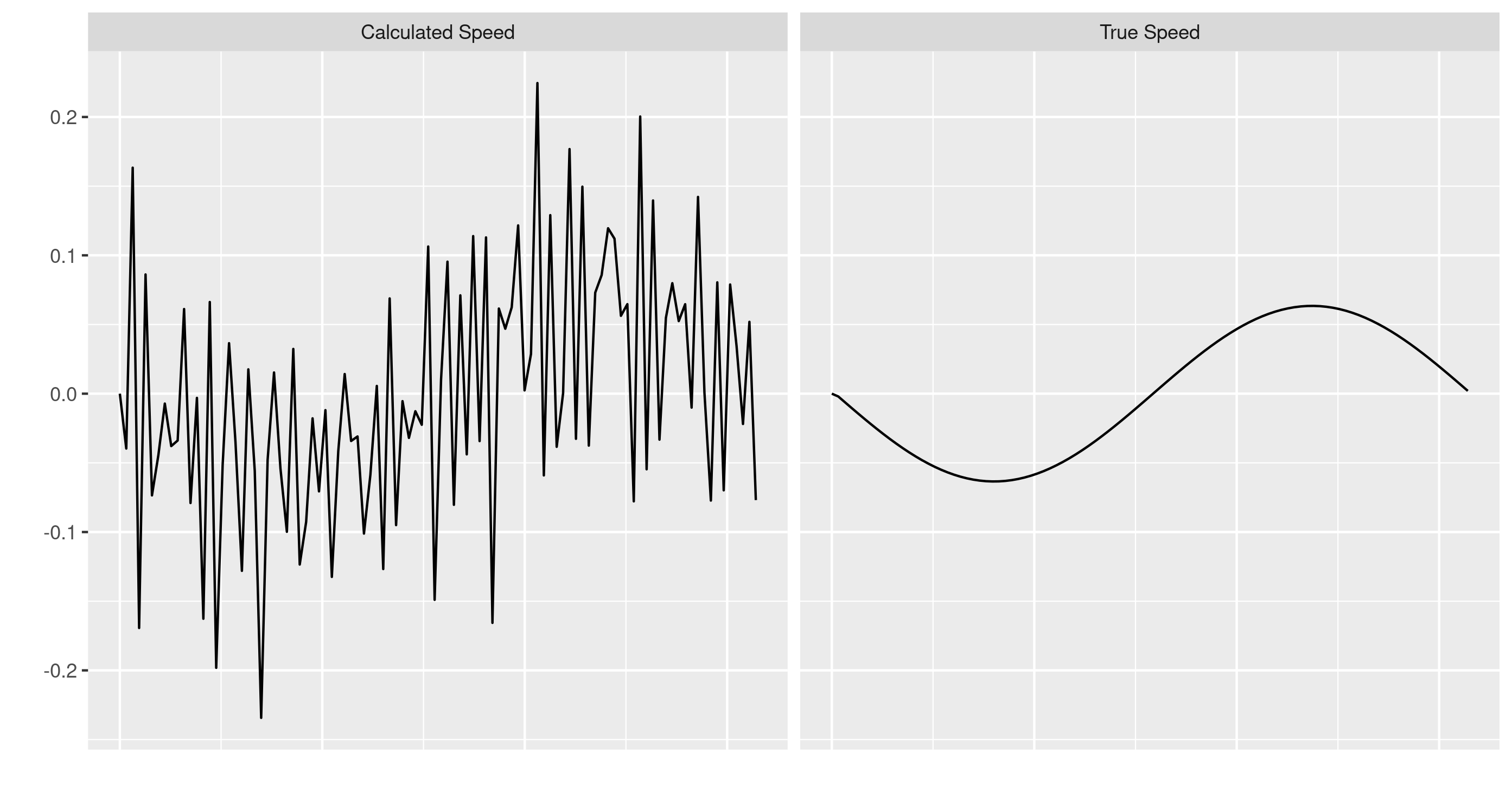
Calculated Speed of the cyclist in the x axis vs True Speed
If we only look at the red GPS readings we do not have a particularly accurate representation of the true path of the cyclist, but in reality we do not measure the true path and will only see the observations from the GPS receiver. We will apply the Kalman filter to these noisy signals to hopefully improve our understanding of the true path of the cyclist.
Kalman Filtering
Health Warning: The following is a fairly heavy look at the individual equations (although this is still not a full derivation!), and is mainly for my own future reference, when we apply it the linear algebra will be followed by the equivalent code in R.
The following section will take each part of the Kalman Filter in turn before relating it to the cyclist example given above.
The State Equation
Kalman filtering fundamentally boils down to two equations, the first determines how our “states”, \(\mathbf{x}_k\), evolve over time:
This equation is better known as the State Equation. This equation models how the vector of true “states” of the system (i.e., the cyclists location, speed, etc.) evolve over time. These true states are unobserved by us (we do not know where the cyclist was exactly at any point in time - we only have the measurements taken from the GPS sensor) and are what we are trying to estimate. The matrix \(\mathbf{A}\) is known as a transition matrix and relates states at time step \(k-1\) to \(k\)). In our example,\(\mathbf{A}\) captures the fact that the location and speed of a cyclist are somehow related to the location and speed of a cyclist a second ago1. The final term, \(\mathbf{w}_k\), is the process noise of the system, a vector of white noise terms with a covariance matrix (i.e., the a matrix which captures the variances on the prime diagonal and the correlations in the off-diagonal elements) defined by \(\mathbf{Q}\). This process noise captures those random fluctuations which impact our true states, for example gusts of wind may randomly impact the speed of the cyclist (although wind is not a great example as it is unlikely to be a true random process).
The Measurement Equation
The second equation is how the observed values (\(\mathbf{z}\)) (i.e., our measured GPS coordinates) are related to the true state values:
This equation is known as the measurement equation. The matrix \(\mathbf{H}\) connects the true states at timestep \(k\), \(\mathbf{x}_k\), to the observations/measurements we have of the system \(\mathbf{z}_k\). At this point it is important to note that the matrix \(\mathbf{H}\) is crucial as the observation vector will often be different to the true states. For example, our cyclist has at least two states we may be interested in: location and speed, however we may only have a GPS device so the measurements only consist of locations. Another example of how \(\mathbf{H}\) may be used is if the measurements need converting into a different unit of the “true” state (for example we may be interested in the speed in miles per hour but have a device which only measures in kilometres per hour). Finally, \(\mathbf{v}_k\) is the measurement noise, a vector of white noise terms with a covariance matrix defined by \(\mathbf{R}\), this is assumed to be independent of the process noise, \(\mathbf{w}_k\), from above. This term captures the fact that there are errors in the observations (for example the GPS errors we discussed above) - Kalman filtering aims to reduce the impact of these measurement errors as much as possible.
Kalman Filter Algorithm
The model presented above is great, except the fact that it is unobservable due to the true states being unknown, so we have to estimate it. To estimate the Kalman Filter we bring everything together in a two step procedure, first a prediction step and then an estimation step. A key idea is that we will make a prediction of what we think the true state will be at the next time period, before correcting it using the new observations of the system. This unfortunately makes the Kalman filter have difficult notation, as we will have an estimate (using standard notation I use hats for estimated values) for the true states before and after corrections are made using the observations in the estimation step. One additional important consequence of this computationally is that we have two different measurements of error, before and after this updating process.
Prediction Step
We begin by predicting the true states of our system and the prediction error covariance matrix (which we will need in a later step) at time period \(k\) given what we the state at the previous time period \(k-1\):
This is where the notation gets more difficult unfortunately. \( \hat{\mathbf{x}}_{k \mid k-1} \) is the estimate of the state vector at time \(k\) given the state at time \(k-1\). During the prediction step, we project forward the current state (\(\hat{\mathbf{x}}_{k-1}\)) using the transition matrix \(\mathbf{A}\) to obtain the estimates for the next time step. (These are sometimes known as a priori estimates if we are being fancy as they are made before we have updated using the measurements we have taken.) At the same time we calculate, \(\mathbf{P}_{k \mid k-1}\), the error covariance matrix of the predictive step using the transpose of \(\mathbf{A}\), \(\mathbf{A}^T\). We now have a prediction of the true states.
Estimation Step
The estimation step updates estimates of the system using the measurements we have taken. First we compute a matrix known as the Kalman gain matrix, \(\mathbf{K}\):
Why this Kalman Gain is calculated this way is a bit out of scope for this current post (this is almost an entire post by itself), however for now I refer you to more in depth derivations such as this introduction. The main intuition to be aware of is that this Kalman Gain matrix is chosen to minimise the posterior error (i.e., the error after the estimation step). Now that we have some predictions for the states we need to evaluate how wrong they are and update the estimates based on new information. We take observations of the system, \( \mathbf{z}_k\), in our case some GPS readings, and update our estimates of the states using a weighted difference between these new observations (\( \mathbf{z}_k\)) and the observation predictions; (\(\mathbf{H}\), the matrix which maps the state onto the observations, multiplied by the results from our predictions of the state)2:
Again if we are being fancy we can say we are generating a set of a posteriori estimates as these estimates are after we have taken observations. Now we have an estimate of the true states with all information up to timestep \(k\). The final step is to update the estimate the a posteriori error covariance:
From the above we can see that for each time step and measurement update we take the estimates from the previous step (posterior estimates) and project/predict them into the future to create the next set a priori estimates. This recursive nature is one of the great things about the Kalman Filter (as compared to other filters such as this which require access to the whole data set) so we can run it in real time as we continue to receive new observations.
I don’t care about theory, show me how to apply it!
So we now have a cyclist travelling around a track with a GPS tracking device. To estimate the Kalman Filter we will need a predictive equation, which we can use relationships defined by the physical system. As with many modelling processes the better our predictive model the better our estimates will be. Given that we know a lot about how cyclists around tracks behave from physics we can produce a very good predictive model. We can model the bikes location (\(x, y \)), its velocity (\(\dot{x}, \dot{y} \)), its acceleration (\(\ddot{x}, \ddot{y} \)) (and could go further and model the jerk3 and the other higher moments) using the following relationships:
The first relationship states that the current position of the cyclist is equal to the previous position of the cyclist, plus the speed (the change of location over time - first derivative of location) the cyclist was going multiplied the the amount of time since the previous step. To this we add terms which capture the cyclists acceleration (the change in speed over time - the second derivative) and the jerk (the change in acceleration over time - the third derivative). Our state vector is \( \mathbf{x}_k = [x,\dot{x},\ddot{x},y,\dot{y},\ddot{y}]^T \), which captures the position, velocity and acceleration. For simplicity we model jerk and the higher order moments as white noise signals \(J_x\) and \(J_y\) in the \(x\) and \(y\) axis respectively which allows us to drop those terms (in reality they get absorbed into our process noise). We can convert the above system of equations into a vector system that will be familiar from the previous discussion:
The \(\bm{A}\) matrix can be constructed in R as follows:
A <- matrix(
  data = c(
    1, dt, (dt**2) / 2, 0, 0, 0,
    0, 1, dt, 0, 0, 0,
    0, 0, 1, 0, 0, 0,
    0, 0, 0, 1, dt, (dt**2) / 2,
    0, 0, 0, 0, 1, dt,
    0, 0, 0, 0, 0, 1
  ),
  nrow = 6, byrow = TRUE
)
Using this model we can get a prediction of where the bike will be at the next time step by plugging in the current estimated values of the state. At this point we should note that although our predictive model will give reasonable predictions one or two steps ahead further into the future it will become increasingly unreliable due to predictive errors - which is where the power of the Kalman filter comes in.
Our observation vector will be just the \(x\) and \(y\) measurements from the GPS receiver, \(\mathbf{z}_k = [x_{\text{GPS}}, y_{\text{GPS}}]^T \). Our \(\mathbf{H}\) matrix just needs to select the \(x\) and \(y\) values from the state vector as we cannot observe the speed or acceleration from location observations:
H <- matrix(c(
  1, 0, 0, 0, 0, 0,
  0, 0, 0, 1, 0, 0
), byrow = TRUE, nrow = 2)
Next we need some estimate for \(\mathbf{Q}\), which is the most ugly looking part of the procedure. \(\mathbf{Q}\) is the error covariance matrix for the process noise in the state equation, \(\mathbf{w}_k\), which in our example will be the third derivative of the cyclist location as chose not to include them in the previous step. We can model these as mean 0 random variables with known variances \(\sigma^2_{J_x}\) and \(\sigma^2_{J_y}\). (In fact as we know the equations of the \(x\) and \(y\) values we can calculate the variance of the third derivatives exactly here):
All of the above variance calculations boil down to the (slightly) nicer looking R code:
# Calculate third derivatives
d3xdt3 <- sin(t)
d3ydt3 <- -cos(t)

# Construct Q vectors
Q1 <- matrix(c((dt^3) / 6, (dt^2) / 2, dt, 0, 0, 0), nrow = 6, byrow = TRUE)

Q2 <- matrix(data = c(0, 0, 0, (dt^3) / 6, (dt^2) / 2, dt), nrow = 6, byrow = TRUE)

# Calculate the variances
sigma2_jx <- var(d3xdt3)
sigma2_jy <- var(d3ydt3)

# Construct Q matrix
Q <- sigma2_jx * (Q1 %*% t(Q1)) + sigma2_jy * (Q2 %*% t(Q2))
The final matrix we need to specify is the error covariance matrix of \(\mathbf{v}_k\), \(\mathbf{R}\). This corresponds to our measurement noise so we model it as a square matrix with the GPS error variances we specified earlier on the diagonal:
# Measurement Error Covariance Matrix
R <- diag(c(gps_sig^2, gps_sig^2))
The last thing we need to specify is some estimates of the cyclists initial states. For simplicity we assume we know the starting location but no knowledge of initial speed or acceleration, and initialise a small prediction error:
# Initial knowledge of State Vector
x_init <- matrix(data = c(x[1], 0, 0, y[1], 0, 0), nrow = 6)

# Initialise Prediction Error
P_init <- 0.01 * diag(1, length(x_init))
Estimate the Kalman Filter
We can now (finally) run the full Kalman Filter using the following R code:
# Observations of the noisy GPS signals
observations <- cbind(x_gps, y_gps)

# Get dimensions of required Matrices
nx <- NROW(Q)
ny <- NROW(R)

# Calculate how many time steps we will be looping through
nt <- NROW(observations)

# Create an Identity Matrix of the appropriate for use in estimation stage
Inx <- diag(x = 1, nx)

# Pre assign some matrices and arrays of the correct size for our application

# Prediction Matrices of state and error covariance
x_pred <- matrix(data = 0, nrow = nx, ncol = nt)
P_pred <- array(data = 0, dim = c(nt, nx, nx))

# Estimation Matrices of state and error covariance
x_est <- matrix(data = 0, nrow = nx, ncol = nt)
P_est <- array(data = 0, dim = c(nt, nx, nx))

# Kalman Gain
K <- array(data = 0, dim = c(nt, nx, ny))

# Initial predictions
x_pred[, 1] <- x_init
P_pred[1, , ] <- P_init

# Step through time
for (i in 1:nt) {

  # Prediction Step
  if (i > 1) {
    x_pred[, i] <- A %*% x_est[, (i - 1)]
    P_pred[i, , ] <- A %*% P_est[(i - 1), , ] %*% t(A) + Q
  }

  # Estimation Step
  y_obs <- observations[i, ]
  K[i, , ] <- P_pred[i, , ] %*% t(H) %*% solve((H %*% P_pred[i, , ] %*% t(H)) + R)
  x_est[, i] <- x_pred[, i] + K[i, , ] %*% (y_obs - H %*% x_pred[, i])
  P_est[i, , ] <- (Inx - K[i, , ] %*% H) %*% P_pred[i, , ]
}
Now that we have run the Kalman Filter we can examine the results:
Comparison of the GPS Signal, Kalman Filtered Signal compared to the True Path of the Cyclist
We can see that the Kalman Filter has taken the noisy signal and converted it to something much closer to the actual true path of the cyclist, all by using known properties of the physical system. In the next blog post I will look at a common extension of the Kalman Filter (the well-named Extended Kalman Filter), which will allow us to incorporate more information we can gather about the cyclists path to make further improvements.
I hope you have found the above description and explanation of the Kalman Filter useful (enjoyable might be a stretch too far). If there are any mistakes they are mine alone, and please feel free to get in touch with any comments or questions using the comments section below. Thanks for reading!
In practice \(\mathbf{A}\) may be time-varying which for simplicity we ignore for now. ↩︎
Those of you who are familiar with exponential smoothing will see a striking resemblance here. ↩︎
Yes, the third derivative of location is really called Jerk, even more amusingly the fourth, fifth and sixth derivatives are sometimes referred to as Snap, Crackle and Pop, who said Physicists had no sense of humour? ↩︎